Visium (HD) Analysis Tutorial
Miranda, Andrew, Francisco, Max, Katarzyna
Last updated: 2025-06-10
Checks: 6 1
Knit directory: VisiumHD_Tutorial/
This reproducible R Markdown analysis was created with workflowr (version 1.7.1). The Checks tab describes the reproducibility checks that were applied when the results were created. The Past versions tab lists the development history.
The R Markdown file has unstaged changes. To know which version of
the R Markdown file created these results, you’ll want to first commit
it to the Git repo. If you’re still working on the analysis, you can
ignore this warning. When you’re finished, you can run
wflow_publish to commit the R Markdown file and build the
HTML.
Great job! The global environment was empty. Objects defined in the global environment can affect the analysis in your R Markdown file in unknown ways. For reproduciblity it’s best to always run the code in an empty environment.
The command set.seed(20250604) was run prior to running
the code in the R Markdown file. Setting a seed ensures that any results
that rely on randomness, e.g. subsampling or permutations, are
reproducible.
Great job! Recording the operating system, R version, and package versions is critical for reproducibility.
Nice! There were no cached chunks for this analysis, so you can be confident that you successfully produced the results during this run.
Great job! Using relative paths to the files within your workflowr project makes it easier to run your code on other machines.
Great! You are using Git for version control. Tracking code development and connecting the code version to the results is critical for reproducibility.
The results in this page were generated with repository version eb68351. See the Past versions tab to see a history of the changes made to the R Markdown and HTML files.
Note that you need to be careful to ensure that all relevant files for
the analysis have been committed to Git prior to generating the results
(you can use wflow_publish or
wflow_git_commit). workflowr only checks the R Markdown
file, but you know if there are other scripts or data files that it
depends on. Below is the status of the Git repository when the results
were generated:
Ignored files:
    Ignored:    .DS_Store
    Ignored:    .Rhistory
    Ignored:    analysis/.DS_Store
    Ignored:    data/.DS_Store

Untracked files:
    Untracked:  figures/
    Untracked:  styles/

Unstaged changes:
    Deleted:    analysis/figures/fig1_topgene.png
    Modified:   analysis/index.Rmd
Note that any generated files, e.g. HTML, png, CSS, etc., are not included in this status report because it is ok for generated content to have uncommitted changes.
These are the previous versions of the repository in which changes were
made to the R Markdown (analysis/index.Rmd) and HTML
(docs/index.html) files. If you’ve configured a remote Git
repository (see ?wflow_git_remote), click on the hyperlinks
in the table below to view the files as they were in that past version.
| File | Version | Author | Date | Message |
|---|---|---|---|---|
| Rmd | eb68351 | kmt555 | 2025-06-07 | update loading info |
| html | eb68351 | kmt555 | 2025-06-07 | update loading info |
| Rmd | b71a5b1 | kmt555 | 2025-06-07 | added info on loading and basic plotting |
| html | b71a5b1 | kmt555 | 2025-06-07 | added info on loading and basic plotting |
| Rmd | 96a3887 | kmt555 | 2025-06-04 | sync |
| html | 96a3887 | kmt555 | 2025-06-04 | sync |
| Rmd | b003646 | kmt555 | 2025-06-04 | sync |
| html | b003646 | kmt555 | 2025-06-04 | sync |
| html | b680c53 | kmt555 | 2025-06-04 | sync |
| Rmd | 65e2d36 | kmt555 | 2025-06-04 | sync |
| html | 65e2d36 | kmt555 | 2025-06-04 | sync |
| Rmd | 03d077d | kmt555 | 2025-06-04 | Start workflowr project. |
contact: tyck@vcu.edu
File creation: June 04, 2025
Update:
Approximate time: 60 - 120 minutes
I. Introduction
1.1. Overview of Spatial Transcriptomics Data
1.2. Objectives
1.3. Requiremnts
##== linux command ==##
...add info here...
II. Data Pre-processing with spaceranger count
If only the molecule_info.h5 file is available, you’ll
need to run spaceranger count to generate the files
required for loading Visium HD data into R or Python.
In this example, Visium HD data files were downloaded from the 10x Genomics website. The following files are needed:
Visium_HD_Mouse_Brain_Fresh_Frozen_molecule_info.h5
Visium_HD_Mouse_Brain_Fresh_Frozen_probe_set.csv
Visium_HD_Mouse_Brain_Fresh_Frozen_spatial.tar.gz
Unpack the spatial image archive using:
##== linux command ==##
tar -xvzf Visium_HD_Mouse_Brain_Fresh_Frozen_spatial.tar.gz
This archive contains a CytAssist image file, which is required for reconstructing spatial coordinates and associating spots with the H&E image.
To run spaceranger count, you must provide the
--slide and --area parameters using the exact
values specified by 10x Genomics for this dataset. These are critical
for mapping spatial barcodes correctly and are typically listed in the
associated metadata or sample sheet.
For this tutorial, the relevant information is:
Slide serial number: H1-7JN9RJG
Area: A-1
Instrument: Visium CytAssist
Probe set: Visium Mouse Transcriptome Probe Set v2.0
Sequencing
Run the following command:
##== linux command ==##
spaceranger count \
  --id=Visium_HD_Mouse_Brain_Fresh_Frozen \
  --transcriptome=../refdata-gex-mm10-2020-A \
  --probe-set=Visium_HD_Mouse_Brain_Fresh_Frozen_probe_set.csv \
  --molecule-h5=Visium_HD_Mouse_Brain_Fresh_Frozen_molecule_info.h5 \
  --image=./spatial/cytassist_image.tiff \
  --slide=H1-7JN9RJG \
  --area=A-1
⚠️ Make sure to adjust the file paths and reference transcriptome directory as needed for your setup.
III. Loading and Visualizing 10x Visium HD Binned Data
10x Genomics now provides binned spatial transcriptomics outputs that allow you to skip the spaceranger count step entirely. You can work directly with the binned data available for download from their website.
✅ This tutorial demonstrates how to load the binned data in R using Seurat v5, and visualize gene expression using SpatialFeaturePlot().
2.1 Download and Unpack Binned Data
10x Genomics (https://www.10xgenomics.com/datasets/) provides preprocessed binned spatial transcriptomics outputs for Visium HD datasets. These files allow you to skip the spaceranger count step entirely.
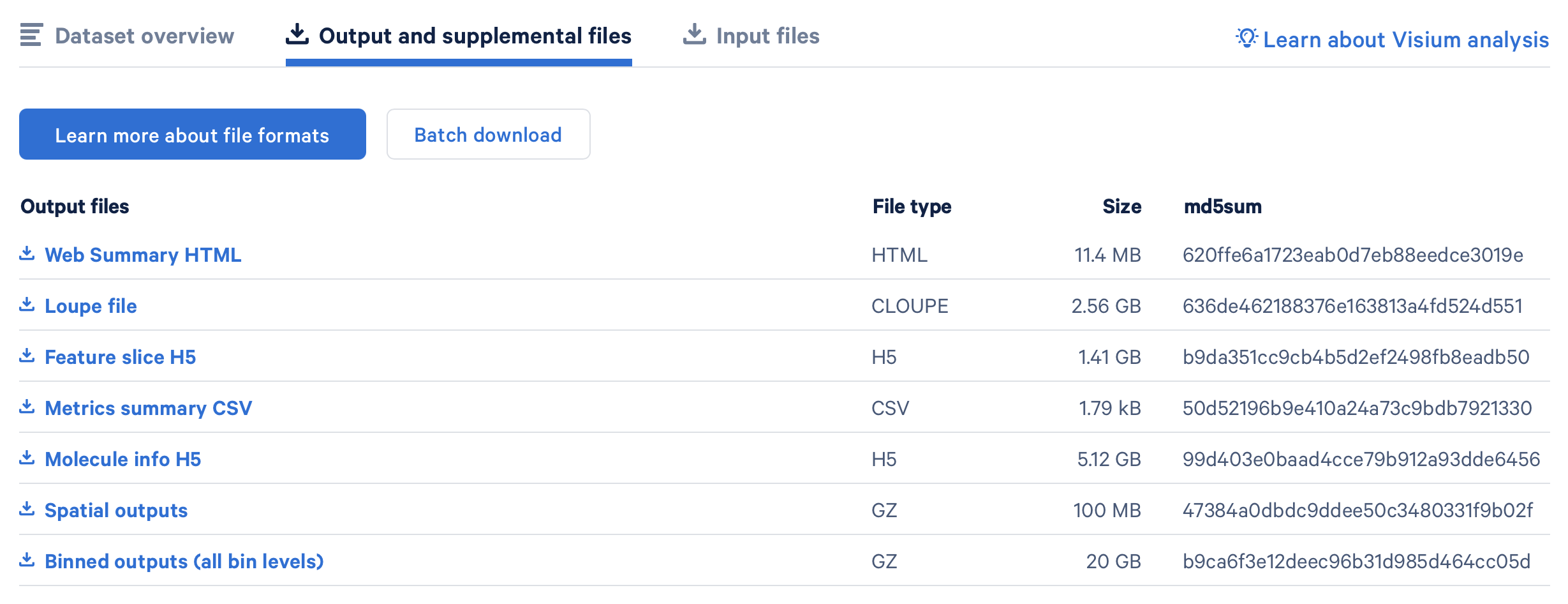
Download Binned outputs (all bin levels)
Once you’ve downloaded and extracted the dataset (e.g., for 8 µm bin resolution), the directory should look like this:
binned_outputs/square_008um/
├── filtered_feature_bc_matrix.h5
├── spatial/
│   ├── tissue_positions.parquet
│   ├── scalefactors_json.json
│   ├── tissue_lowres_image.png
│   ├── aligned_fiducials.jpg
│   ├── aligned_tissue_image.jpg
│   ├── cytassist_image.tiff
│   ├── detected_tissue_image.jpg
│   └── tissue_hires_image.png
This directory contains everything needed to load the dataset into Seurat v5 for downstream analysis and visualization.
2.2 Load and Normalize the Data in R
library(Seurat)
library(ggplot2)
library(dplyr)

# Load the Visium HD binned data
seurat_obj <- Load10X_Spatial(data.dir = "./binned_outputs/square_008um/")

# Normalize the data to create the 'data' slot used for plotting
seurat_obj <- NormalizeData(seurat_obj)

top_genes <- rowSums(seurat_obj@assays$Spatial@counts) %>%
  sort(decreasing = TRUE) %>%
  head(20)

top_gene <- names(top_genes)[3]  # Change index to explore other genes

SpatialFeaturePlot(
  seurat_obj,
  features = top_gene,
  images = NULL,            # remove the H&E image
  pt.size.factor = 2        # larger spots
) +
  ggtitle(paste("Top expressed gene:", top_gene)) +
  scale_fill_gradient(low = "white", high = "purple4")
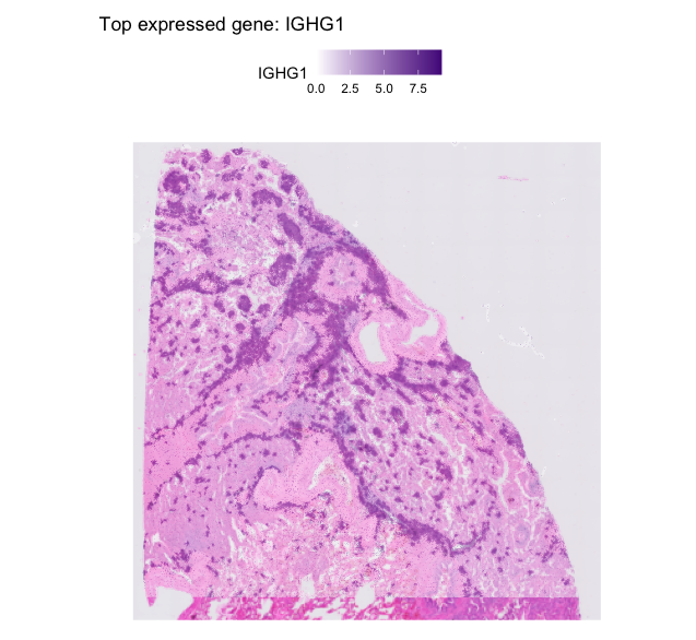
Figure 1. Visualization of Top Expressed Gene. Example visualization of a highly expressed gene across spatial bins, displayed using a single-color gradient ranging from white to a saturated hue. This approach highlights spatial expression patterns while maintaining sensitivity to low-abundance signals.
| Version | Author | Date |
|---|---|---|
| b71a5b1 | kmt555 | 2025-06-07 |
2.3. Quality Control
SpatialFeaturePlot(seurat_obj, features = "nCount_Spatial") +
  ggtitle("Total UMI counts per bin") +
  scale_fill_gradient(low = "white", high = "purple4")
III. Dimensionality Reduction and Clustering
seurat_obj <- FindVariableFeatures(seurat_obj, selection.method = "vst", nfeatures = 2000)
head(VariableFeatures(seurat_obj), 20)
IV. Cell Typing
V. Advanced: Overlaying with Bacterial Load
VI. Gene Expression Analysis in Spatial Context
VII. Additional Tutorials
VIII. References
sessionInfo()R version 4.4.0 (2024-04-24)
Platform: aarch64-apple-darwin20
Running under: macOS 15.5
Matrix products: default
BLAS: /Library/Frameworks/R.framework/Versions/4.4-arm64/Resources/lib/libRblas.0.dylib
LAPACK: /Library/Frameworks/R.framework/Versions/4.4-arm64/Resources/lib/libRlapack.dylib; LAPACK version 3.12.0
locale:
[1] en_US.UTF-8/en_US.UTF-8/en_US.UTF-8/C/en_US.UTF-8/en_US.UTF-8
time zone: America/New_York
tzcode source: internal
attached base packages:
[1] stats graphics grDevices utils datasets methods base
other attached packages:
[1] workflowr_1.7.1
loaded via a namespace (and not attached):
[1] vctrs_0.6.5 httr_1.4.7 cli_3.6.5 knitr_1.50
[5] rlang_1.1.6 xfun_0.52 stringi_1.8.7 processx_3.8.4
[9] promises_1.3.3 jsonlite_2.0.0 glue_1.8.0 rprojroot_2.0.4
[13] git2r_0.36.2 htmltools_0.5.8.1 httpuv_1.6.16 ps_1.7.6
[17] sass_0.4.10 rmarkdown_2.29 jquerylib_0.1.4 tibble_3.2.1
[21] evaluate_1.0.3 fastmap_1.2.0 yaml_2.3.10 lifecycle_1.0.4
[25] whisker_0.4.1 stringr_1.5.1 compiler_4.4.0 fs_1.6.6
[29] pkgconfig_2.0.3 Rcpp_1.0.14 rstudioapi_0.16.0 later_1.4.2
[33] digest_0.6.37 R6_2.6.1 pillar_1.10.2 callr_3.7.6
[37] magrittr_2.0.3 bslib_0.9.0 tools_4.4.0 cachem_1.1.0
[41] getPass_0.2-4